Intrusion of Personal Space as a Cause for Violence: An Inverse Reinforcement Learning Problem on Laboratory Mice

This is the final project I delivered for the COGS566 Probabilistic Models of the Mind course I took during the Fall 2021 semester. This is was a course project of two parts, a literature review and a final report, which I present here. The goal of the project was to make use of probabilistic programming to solve a cognitive science-related problem. I chose the problem and the dataset myself, made the literature review, designed the model and trained it in WebPPL. Despite my best efforts, my model did not work (learn), and so I accepted my fate and decided to write something like a negative result report. I wasn’t very optimistic about it because of this failure, but the positive feedback I received from my instructor, Barbaros Yet, makes this project dear to me. I learned that analysing a model that does not work is a part of scientific process and to value negative results.

Abstract

This project aims to explain how the intrusion of an agent’s personal space can cause the agent to act aggressively. The data used are of laboratory mice and is collected from the CalMS21 dataset. A linear utility function specific to each action is assumed, and their parameters are attempted to be learned by a model written in the probabilistic programming language WebPPL. The model in this project fails to make the desired link, so the results remain inconclusive.

Keywords: aggression, territoriality, inverse reinforcement learning, laboratory mice, WebPPL

Introduction

Intrusion of personal space is a phenomenon to which we are well accustomed from our day-to-day lives: It has the potential to occur in almost all public spaces and during many communications in person. In this project, I wanted to explore this familiar experience in a more quantitative manner. Using a dataset on laboratory mice, I aimed to explore the physical cues that lead to aggression. I formulated the problem as an Inverse Reinforcement Learning Model, where the task is to learn the utility function of an agent given their actions, and attempted to solve it within the Bayesian inference framework using probabilistic programming.

Outline. The report is organized as follows: In the following subsection, I will give some background very briefly, regarding aggression and territoriality in laboratory mice and IRL on animal modelling.¹ Then, I will go through my methodology in the next section, focusing on the dataset, data preprocessing, and modelling. I will analyse my results and evaluate the success of my process in the proceeding section and then in the final section conclude by discussing the overall results of my work and conclude.

Background

Although behavioural analyses of laboratory are important in their own right, the understanding their behavioural patterns is also important for more practical and experimental reasons. Mackintosh (1970) in their work make various experiments on laboratory mice to discover whether these animals are territorial, and under which circumstances they choose to attack. They revealed that especially male mice enclosed in a common space will tend to attack one another until one establishes dominance over a territory, and even after then the dominant mouse patrols the area and keeps the others in check by chasing and attacking them. Juvenile and female mice, however, seem to be exempt from the violence of the territorial male mice.

Inverse Reinforcement Learning (IRL) is the process of learning the utility function of an agent, based on their observed actions in an environment (Ng, Russell, et al., 2000). Yamaguchi et al. (2018) in their work apply this framework to the C. Elegans worm, due to the animal’s simplistic nature. They record the behaviour of 80-150 worms in agar with controlled temperature gradients. The state model is rather simple with only two dimensions, the current temperature and its temporal derivative. Their model consists of two actions, “passive behaviour” denoting the involuntary drift of the animal in the environment and “reward-maximizing behaviour” being the being the voluntary turns and movements to direct its movement towards a reward source (such as food). They model this behavioural strategy using the analytical solution to a linearly-solvable Markov decision process (LMDP), which requires a value function, which they aim to extract from the worms recorded behaviour.

These two works provide the basis on which I build my model: The work of Mackintosh asserts that laboratory mice are indeed territorial, so they will attack to protect what would be their “personal space”, and the work of Yamaguchi et al. both provides a framework to work in and proves that IRL can successfully be applied to model animal behaviour, although I am working with much more complex animals compared to theirs.

Method

Broadly speaking, the data processing pipeline I followed was as follows:

1. Importation the dataset into a Python notebook on Google Colab.
2. Elementary preprocessing on the raw data.
3. Feature extraction using NumPy (Harris et al., 2020).
4. Exportation of the data in JSON format for importation to WebPPL (Goodman & Stuhlmüller, 2014).
5. Model training and result acquisition in WebPPL.
6. Analysis of model training results in Python back in Colab.

I chose to use WebPPL only for model fitting purposes, as I found Python to be a better environment for data visualization, processing, and analyses in general.

Dataset. The data is taken from the Caltech Mouse Social Interactions (CalMS21) Dataset, which aims to provide data for multi-agent behaviour modelling in neuroscience (Sun et al., 2021). The dataset contains various subsets belonging to different tasks, but in this work I only used Task 1 data, so the following descriptions are to be read with this consideration in mind.

The raw data of the experiment is collected with a camera at a bird’s eye view of a mouse enclosure. One male mouse, called the resident mouse, is habituated to the enclosure first. Then, another white intruder mouse is introduced into the cage. Their interactions are recorded by the top-mounted camera with a 30 Hz frame rate. Each frame is then given one of these four labels by experts describing which action is being performed by the resident mouse: Attack, investigation, mounting, and other. The distinguishing feature of this dataset is that along with the videos of the recordings, time series describing the seven anatomically chosen points on each mice is provided. Each frame is processed using Mouse Action Recognition System (MARS) software (Segalin et al., 2021) which makes use of recent advances in computer vision to extract these seven points. Figure 1 shows a summary of the experiment setup and the information provided by MARS.

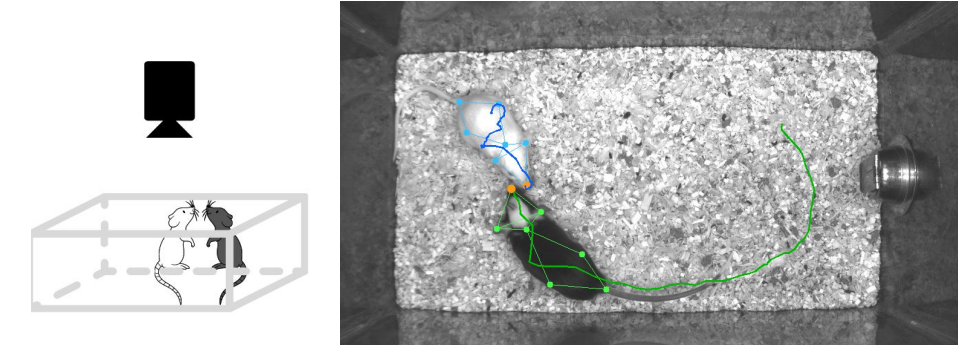
Figure 1: (Left) A simplified schematic of the experiment setup. (Right) A sample frame from the recordings, together with the pose estimates from MARS and a trail left by each mouse. Picture taken with modifications from Sun et al. (2021).

The data as imported via the code provided in Behavior Classification Starter Kit (n.d.), contains 70 measurement sets from the same annotator. Each measurement is a dictionary object, containing

• annotations describing the action of the resident mouse,
• keypoints, a NumPy array of dimensions (# frames) $\times$ (mouse ID) $\times$ ($x$, $y$ coordinate) $\times$ (body part), where \begin{itemize}
  • the resident mouse is indexed by 0 and the intruder mouse is indexed by 1.
  • body parts are numbered from 0 to 6 in the following order: nose, left ear, right ear, neck, left hip, right hip and base of the tail.
  • the $x$ and $y$ coordinates are given as integers denoting pixels in $1024 \times 570$ images.
• metadata describing the annotator and the annotation vocabulary.
• scores, a NumPy array of dimensions (# frames) $\times$ (mouse ID) $\times$ (body part), describing the confidence estimates of each point on each mouse as provided by MARS.

Preprocessing. The only preprocessing applied to the data is median filtering, which is a basic method of noise removal (Davies, 2004). I opted for this preprocessing step due to its simplicity, and the heavy noise I observed upon plotting the location of each mouse, which showed quite unrealistic, sudden jumps. I deemed that they are likely due to MARS and not the mice themselves. Figure 2 shows the data after this median filtering.

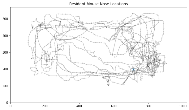
Figure 2: Resident mouse nose locations after median filtering. The initial point is marked with a blue cross. Data taken from the fifth training data.

Feature Extraction. To keep the model simple, only the three features are extracted from the data. The three are put in a three dimensional list as a state vector, which contains the following information in the given order:

• Euclidean distance of the intruder’s nose to the resident’s.] This is used a sa proxy for the distance between the two mice as perceived by the resident mouse. The obtained values are normalized by the diagonal length of the frame. If $l_r^{(nose)}$ and $l_i^{(nose)}$ denote the nose locations of the resident and intruder mice, the obtained state, say $x_t$ at time $t$ is proportional to $|l^{(nose)}_r - l^{(nose)}_i|_2$.

• Approach velocity of the intruder’s nose to the resident.] This value is approximated from the previous state using the constant velocity model:

  \[v_t = \frac{x_{t+1} - x_t}{\Delta t}\]

  where $\Delta t$ is the sampling frequency of the camera, equal to $1 / 30$ seconds. Because this is computed from an already-normalized quantity, I applied no further normalization.

• Cosine of the angle between the orientations of the two mice.] This value is found for each time frame using the head orientations of the two mice. Let $\vec{h_r}$ and $\vec{h_i}$ denote the head vectors of the resident and intruder mice, respectively, each found by \(\vec{h_r} = l^{(nose)}_r - l^{(neck)}_r \qquad \vec{h_i} = l^{(nose)}_i - l^{(neck)}_i\) where $l^{(neck)}$ denotes neck location of each mice. The cosine of the angle between these two vectors at time $t$ is then computed as

  \[\cos\theta_t = \frac{\vec{h_r} \cdot \vec{h_i}}{\|\vec{h_r}\|_2\|\vec{h_i}\|_2}\]

  I opted for the cosine of the angle and not the angle directly as it was a symmetric measure around 0 naturally.

Therefore at each $t$, the state $[x_t, v_t, \cos\theta_t]$ is provided to the model, along with the behaviour annotations.

Model. I wrote the model in WebPPL (Goodman & Stuhlmüller, 2014) to make use of the probabilistic programming facilities. I wrote a sequential inferencing algorithm, where the prior is provided only in the beginning, each time instance is processed on its own and the posterior is provided as a prior to the next datum of time instance.

The state transition model is taken as the constant velocity model, and the third state is always assumed to be constant:

The other two states are taken to be constant. This transition function is cached to save on computation time, which is why it is left deterministic.

The mouse model uses an affine function to evaluate the instantaneous utility of each action. For an action $a$, the instantaneous utility is

where the coefficients $\alpha^a_i$ are specific to each action, which are the quantities to be inferred. The cumulative utility is the discounted sum of future utilities. The future utilities are computed using the transition function given above. The mouse is coded as a maximum utility agent, so the action that brings the maximum utility is selected deterministically.

The linear utility functions are kept reserved for meaningful actions, like attacking and investigation. The utility of taking no actions is fixed at 0. Future utilities $k$ step ahead of current time are discounted by the discount factor $\gamma^k$, where $\gamma = 0.9$. Finally, the infinite recursion is approximated by a finite one, with maximum recursion depth equal to 10.

For all the parameters $\alpha^a_i$ to be inferred, an uncorrelated multivariate gaussian with marginal variances of 15 with zero mean is used.

Results

The initial results of the inference process seemed like a success in the beginning, as the model seemed to be learning some non-trivial parameters. But later on, I realized that different runs of the model with the same dataset inferred radically different coefficients. Additionally, each inference session resulted in a deterministic result, meaning the posterior distribution turned out to be a probability mass function concentrated on a single point in the parameter space.

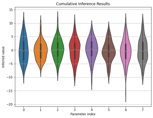
Figure 3: Indices on the $x$-axis show the parameter indices, where the first four belong to the attack utility coefficients, the later four are the investigation utility coefficients.

Figure 3 shows violin plot of the cumulated inference results over a single data time series. The fifth training data in Task 1 is used over 100 inferencing sessions. As it can be seen on the plot, the inferred parameters reflect the prior and not the data, each parameters reflecting a zero-mean Gaussian of variance 15.

To prevent both of these phenomena, namely of collapsing posteriors and the fact that the algorithm was not making proper inferencing, I made use of difference algorithms within WebPPL, none of which made a difference.

I passed on to approximate inferencing to hopefully avoid these situations. After each one-step inferencing using a single data point, I approximated the distribution with a Gaussian by matching the means and standard deviations, which then became the prior for the next data point. With this, I aimed two things:

• I wanted to prevent the posteriors from collapsing onto a single point in the parameter space. To do so, I checked the standard deviations of each parameters, and reset the ones who fall below a certain threshold. Such checks and heuristic manipulations are applied in various algorithms, e.g. Expectation-Maximization (Bishop, 2006).
• I also hoped that sampling from a primitive distribution, the Gaussian here, would prevent the learning process from failing.

During each inference session, I checked the means and standard deviations at regular intervals. Those results looked promising on their own, as the means seemed to move around in the beginning and settling on a value after some amount of data has been processed and the standard deviations gradually decreased, and even the resetting them did not affect their corresponding means.

Despite these preventions, the learning process did not improve. As the results are very similar to the one depicted in Figure 3, I will not give any more examples to avoid redundancy.

Discussion

I classify my reasons for my model’s failure under various categories.

Failure in State Modelling. Intrusion of the resident mice’s cage does not always result in attacking behaviour: There are numerous time series where no attacking happens, or even attacking behaviour is exhibited along with mounting, which can be considered as sexual or affectionate behaviour. However, in general, one of the authors of the work by Sun et al. (2021) expressed that the ones with violent (or frequent, looking at the data only) attacks are the ones where the intruder mouse is male, and the ones without have female intruders. This suggests that attacking behaviour is not induced by the sheer intrusion of space, but dominantly induced by the intruder mouse’s sex. In such a case, which I believe is most likely especially given the literature review, there would be little to no correlation between the resident mouse’s attacking or mounting behaviour and the spatial state variables I choose. The complexity of laboratory mice’s behaviour may have been too complex to be captured in my simplistic model.

Failure in Utility Function. I applied IRL within the Bayesian setting to learn the utility function of the resident mice, and I assumed an affine utility model. This may fail to capture the intricacies of the actual model, which may depend on other variables than the ones I define, or even depend differently on the ones I do define. I have experimented with a quadratic utility using only the $x_t$ and $v_t$ variables, but those results were again inconclusive, i.e. were distributed according to the prior. This trial, however, is obviously not exhaustive: It is possible that there is a possible set of spatial features that can be extracted from this dataset that would describe the resident mouse’s behaviour successfully.

Lack of Information Transfer. The current model does not transmit the next state estimate or the action taken at one time instance to then next and the state transition function takes no action into account, which are common-found properties in reinforcement learning models. Perhaps a model that transmits also the taken action into the next data point and a better state transition model that is also action dependent would result in better inference.

Deterministic vs. Stochastic Modelling. My model here is a deterministic model, i.e. a maximum utility agent that always choses the maximum utility action. However as we have seen in the lectures as well, this need not model an observed agent’s behaviour. A softmax agent with some stochasticity in its action choices could have performed well, partly due to the additional randomness in the action selection process.

Conclusion

In this study, I tried to learn the utility function of a mouse from the data in the CalMS21 dataset. I made use of an affine utility function over a set of spatial variables to see which spatial features of the intruder cause the resident to mainly attack, but also cause other behaviours as well. The results of my project remain inconclusive. The model as it is implemented in WebPPL failed to successfully learn such a utility function. In the end, I discuss the possible technical reasons for my model’s failure, which are failures in the model and hence the modeller. Perhaps a different model and modeller can come up with a better methodology to come and make the desired link, between the spatial features of an intruder and its effects on resident aggression.

Supplementary Material: Data and Code

The supplementary material for this project are given here in GitHub. Supplementary Material A is a .ipynb file, which is the Google Colab notebook I use and a .md document, which is the WebPPL notebook. The Google Colab notebook contains the necessary code snippets that download, processes and exports the data in JSON format. The JSON file is not absolutely necessary, as the WebPPL notebook already contains it as a string. Supplementary Material B is the WebPPL notebook containing the model, it prints out the results in an array format to be analysed back in Colab for the non-approximated case. The models with the approximated distributions are left as they are, without multiple inference sessions.

Notes

1. I kept this section as short as reasonably possible, as I already made an exposition of these works in a previous literature review assignment. Back up.

References

Behavior classification starter kit. (n.d.). Neuromatch Academy. Retrieved from https://colab.research.google.com/github/NeuromatchAcademy/course-content/blob/master/projects/behavior/Loading_CalMS21_data.ipynb

Bishop, C. M. (2006). Pattern recognition. Machine learning, 128(9).

Davies, E. R. (2004). Machine vision: theory, algorithms, practicalities. Elsevier.

Goodman, N. D., & Stuhlmüller, A. (2014). The Design and Implementation of Probabilistic Programming Languages. http://dippl.org. (Accessed: 2022-1-31)

Harris, C. R., Millman, K. J., van der Walt, S. J., Gommers, R., Virtanen, P., Cournapeau, D., … Oliphant, T. E. (2020, September). Array programming with NumPy. Nature, 585(7825), 357–362. Retrieved from https://doi.org/10.1038/s41586-020-2649-2 doi: 10.1038/s41586-020-2649-2

Mackintosh, J. (1970). Territory formation by laboratory mice. Animal Behaviour, 18, 177–183.

Ng, A. Y., Russell, S. J., et al. (2000). Algorithms for inverse reinforcement learning. In ICML (Vol. 1, p. 2).

Segalin, C., Williams, J., Karigo, T., Hui, M., Zelikowsky, M., Sun, J. J., … Kennedy, A. (2021). The mouse action recognition system (mars) software pipeline for automated analysis of social behaviors in mice. Elife, 10, e63720.

Sun, J. J., Karigo, T., Chakraborty, D., Mohanty, S. P., Wild, B., Sun, Q., … Kennedy, A. (2021). The multi-agent behavior dataset: Mouse dyadic social interactions. arXiv preprint arXiv:2104.02710.

Yamaguchi, S., Naoki, H., Ikeda, M., Tsukada, Y., Nakano, S., Mori, I., & Ishii, S. (2018, 05). Identification of animal behavioral strategies by inverse reinforcement learning. PLOS Computational Biology, 14(5), 1-20. Retrieved from https://doi.org/10.1371/journal.pcbi.1006122 doi: 10.1371/journal.pcbi.1006122