A novel approach to characterizing the visual dimensions of mental imagery vividness using Gaussian process regression
Published in Vision Sciences Society Annual Meeting, 2026
Recommended citation: A novel approach to characterizing the visual dimensions of mental imagery vividness using Gaussian process regression (2026) Yurdakul O.C., Huang X., Shen A., Olsson E., Ekhlasi A., Klímová M., Morales J.*, Peters M.A.K.* Vision Sciences Society Annual Meeting https://www.visionsciences.org/presentation/?id=4213
Poster Supplements - Last updated: 2026.06.06
This is a living document where I will add any supplementary information/results about my poster, which you can find here.
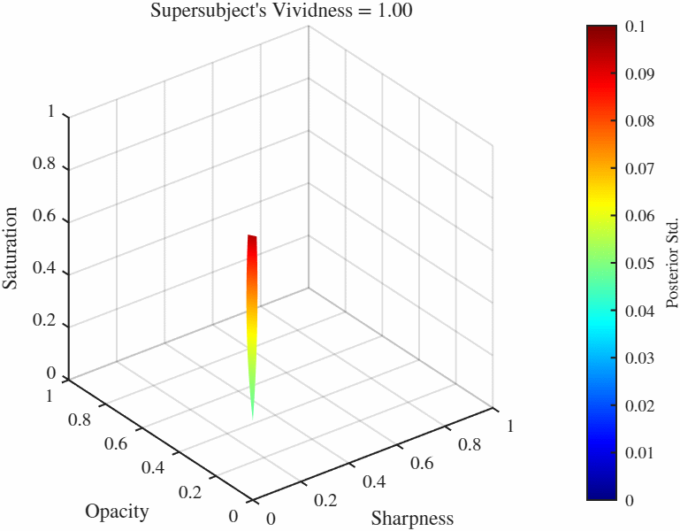
Animated Manifolds Equal vividness manifolds: These are sets of points in the feature space $[0, 1]^3$ that result in identical vividness ratings in a specific GP. This list has manifolds from each cluster.
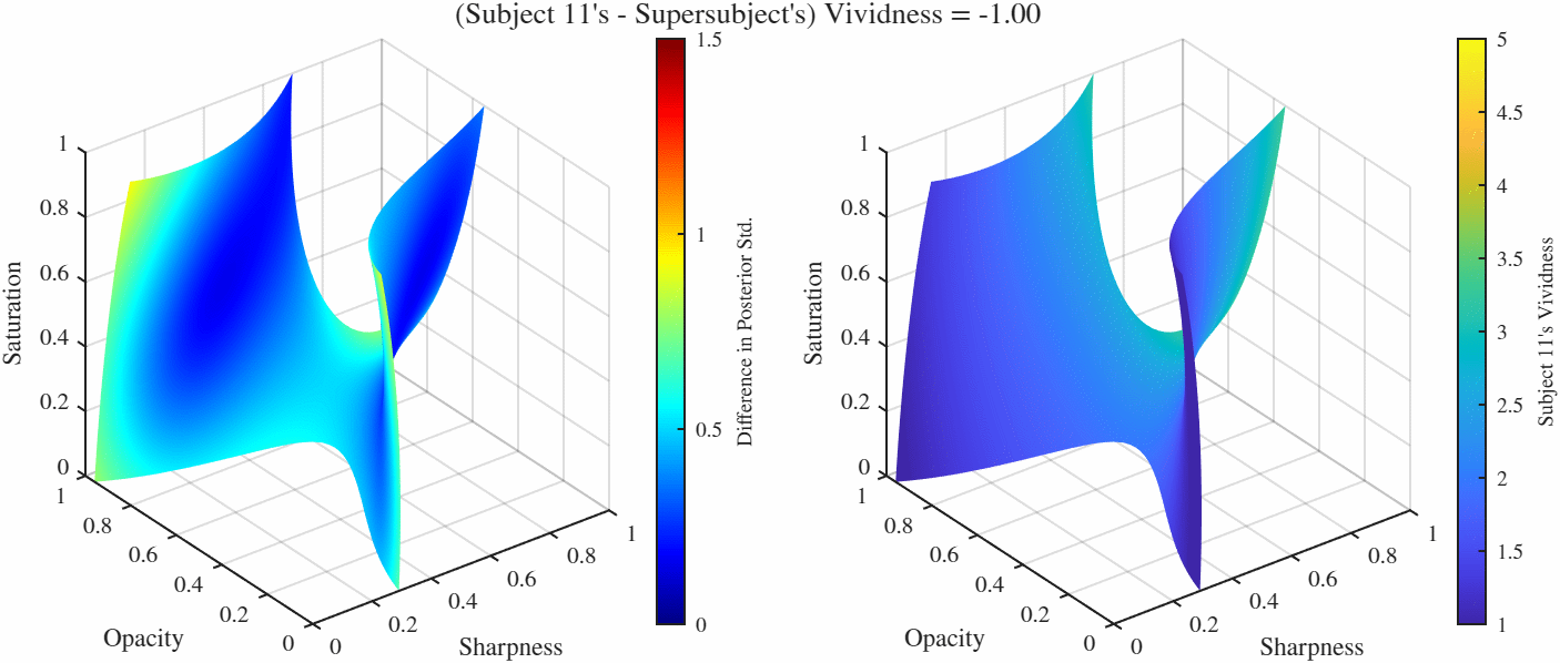
Difference manifolds: These are sets of points in the feature space $[0, 1]^3$ that result in constant *difference* between two GPs, here these are the differences between the representative subjects from each manifold and the supersubject. Because in this case we have two manifolds, there is more than one way to folor the manifolds: We can either color if by the difference of posterior standard deviations occurring at over the manifold which tells us the how the confidence ratings differ over those points, or we can color by the function value (i.e. the vividness rating) of one of the manifolds. Here we color both by the difference of posterior standard deviations (left) and the vividness rating at the supersubject (right). One particularly useful manifold is when the difference is set to 0, gives us the manifold over which two functions agree. Therefore if we would like to find the point(s) that elicit a particular vividness rating for two subjects (or more interestingly as a subject and the overall population as represented by the supersubject), we go to the 0-difference manifold and set the vividness level (which will likely) give us a curve (more technically a 1-D manifold in this case). We can then further minimize the standard deviation over this reduced manifold as well.
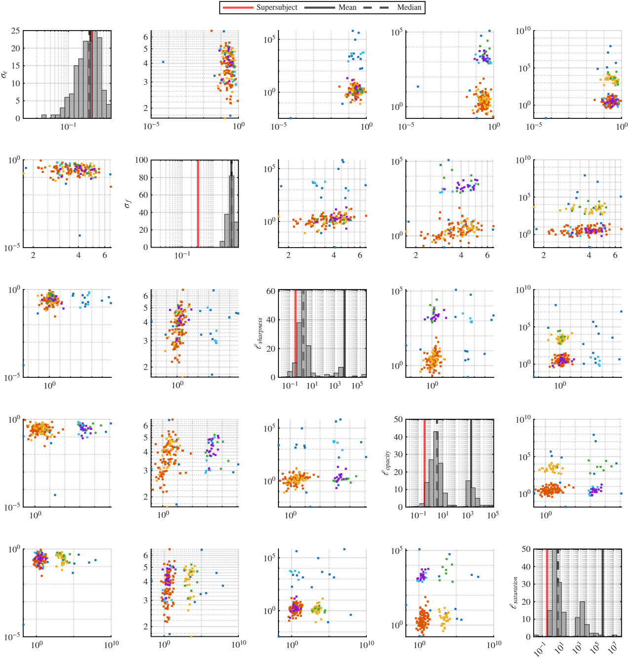
Clustering Results These are the pair-wise scatter plots of the hyperparameters of each subject along with the histograms. The histograms also show the supersubject hyperparameters, which are obtained by treating as if all the data came from a single "super"subject and optimizing the hyperparameters over that space. We can see that while the noise standard deviation is pretty typical of among the subjects, the length scales are significantly lower and the signal standard deviation is significantly higher. We believe that this is due to the mixing of single-subject noise variances into a single data pool.
Agreement with Previous Findings
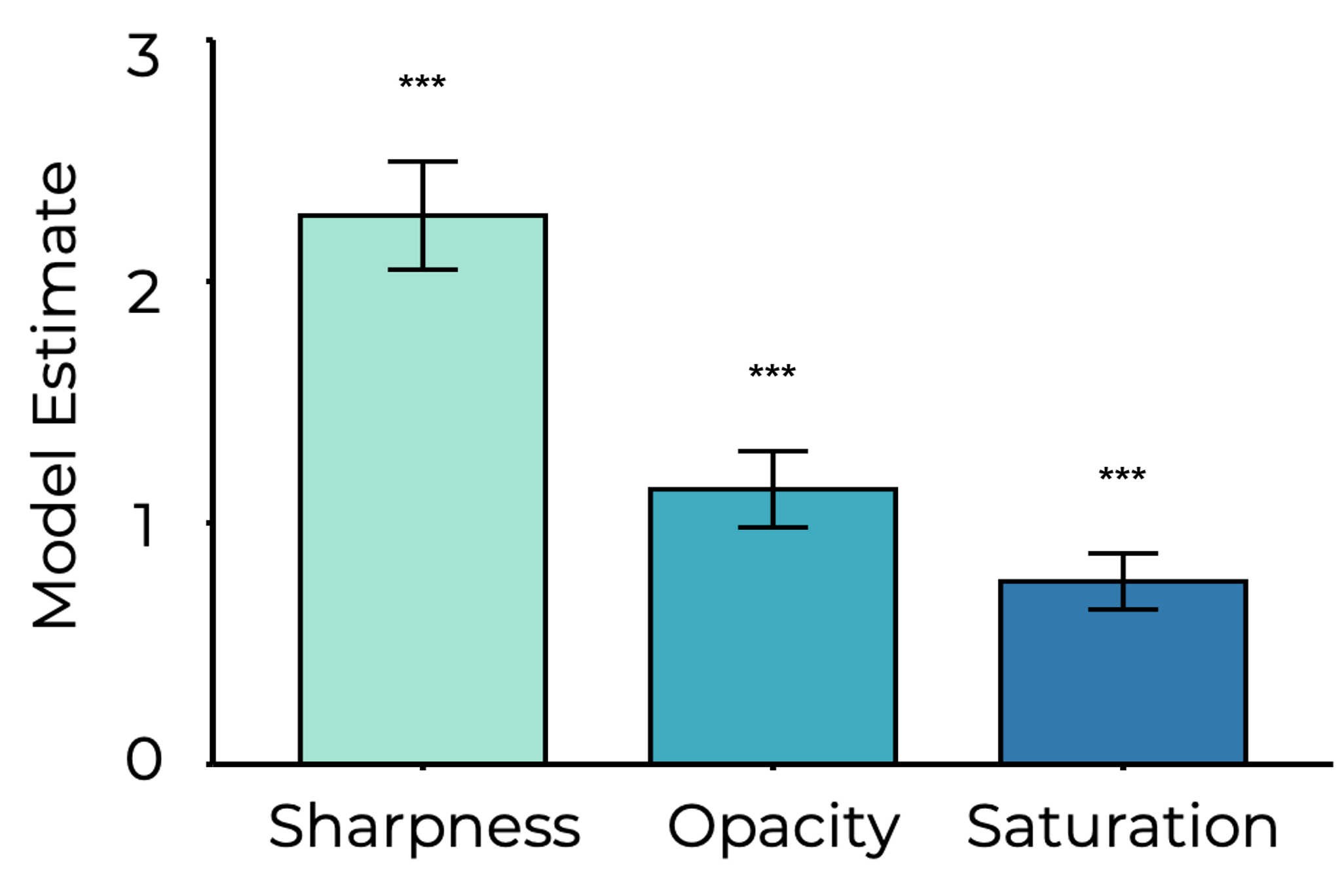
Previous findings as depicted in Huang et al. (2025)
Huang et al. (2025) found that sharpness was the most prominent feature, followed by opacity and with saturation being the least prominent. We can see this finding replicated in the manifolds: The fact that equal vividness manifolds usually span the whole saturation axis and are narrow on the sharpness axis is agreeing with these results. Gaussian Processes A Gaussian process (GP) is a collection of random variables such that any finite collection of them has a jointly Gaussian distribution, so is completely specified by its mean and covariance. For a real-valued GP function $f(\vec x)$, denoted $f(\vec x) \sim \mathcal{GP}\left(m(\vec x),\, k(\vec x, \vec x')\right)$, the mean and covariance functions are defined as $$ \begin{align} m(\vec x) &= \mathbb E\left[f(\vec x)\right] \\ k(\vec x, \vec x') &= \mathbb E \left[\left(f(\vec x) - m(\vec x)\right)\left(f(\vec x') - m(\vec x')\right)\right] \end{align} $$ where $k(\vec x, \vec x')$ is called the kernel function. To formulate the regression setting, let $f$ be an unknown function from which we obtain observations $y_i$ at input locations $\vec x_i$ for $i = 1, ..., N$, via the noisy model $$ y_i = f(\vec x_i) + \epsilon_i $$ where $\epsilon_i \sim \mathcal{N} \left(0,\, \sigma_\epsilon^2\right)$ is the independent identically distributed additive noise and $f$ is the unknown function of interest. Within the GP regression framework, $f$ is taken to be a GP independent of $\epsilon$, commonly with prior mean 0 for convenience. This allows us to take an arbitrary query location $\vec x^\ast$ at which we would like to estimate the function value, and write the joint distribution $$ \begin{bmatrix}f(\vec x^\ast) \\ \vec y \end{bmatrix} \sim \mathcal{N}\left(\begin{bmatrix}0 \\ \vec 0\end{bmatrix},\, \begin{bmatrix}k(\vec x^\ast, \vec x^\ast) & k(\vec X, \vec x^\ast)^{\intercal} \\ k(\vec X, \vec x^\ast) & k(\vec X, \vec X) + \sigma_\epsilon^2 I_N\end{bmatrix}\right) $$ where $\vec y$ denotes the vector of noisy observations, $k(\vec X, \vec x^\ast)$ denotes the column vector of cross correlations $k(\vec x^\ast, \vec x_i)$, $k(\vec X, \vec X)$ denotes the correlation matrix with entries $k(\vec x_i, \vec x_j)$, and $I_N$ is the identity matrix of size $N$. By the Gaussian conditioning rule, the conditional distribution of $f(\vec x^\ast)$ on the observations becomes $\mathcal{N}\left(\mu(\vec x^\ast),\, \sigma^2(\vec x^\ast)\right)$ where $$ \begin{align} \mu(\vec x^\ast) &= k(\vec X, \vec x^\ast)^{\intercal} \left[ k(\vec X, \vec X) + \sigma_\epsilon^2 I_N \right]^{-1} \vec y, \\ \sigma^2(\vec x^\ast) &= k(\vec x^\ast, \vec x^\ast) - k(\vec X, \vec x^\ast)^{\intercal} \left[ k(\vec X, \vec X) + \sigma_\epsilon^2 I_N \right]^{-1} k(\vec X, \vec x^\ast). \end{align} $$ The choice of a kernel function is essential for GPs since it determines the form and properties of the function $f$. One commonly used kernel function (and the one used in this work) is the squared exponential kernel, defined as $$ k(\vec x, \vec x') = \sigma_f^2 \exp\left(-\frac{\|{\vec x - \vec x'\|^2}}{2\ell^2}\right) $$ where the signal variance $\sigma_f^2$ and the length-scale $\ell$ are hyperparameters of interest. One assumption of this kernel function is that it effectively assumes that the correlation structure is identical across the dimensions of $\vec x$, which need not be true in general. One improvement/generalization we can make is to have separate length scales for each dimension, which gives us the kernel function $$ k(\vec x, \vec x') = \sigma_f^2 \exp\left(\frac{-1}{2} \sum_{d = 1}^D\frac{(\vec x_{(d)} - \vec x'_{(d)})^2}{\ell_{(d)}^2}\right) $$ where $\ell_d$ is the length scale corresponding to the feature $d$ and $d = 1,..., D$ indexes the dimensions of the feature vector $\vec x \in \mathbb R^D$. Having different length scales like this allows us to assess how much each feature contributes to the posterior: If a length scale is too large (with respect to the interval of interest), then it means that a change along that feature will not correspond to a change in the posterior function value significantly.